Compositional data
Parts of a whole which carry only relative information
From Wikipedia, the free encyclopedia
In statistics, compositional data are quantitative descriptions of the parts of some whole, conveying relative information. Mathematically, compositional data is represented by points on a simplex. Measurements involving probabilities, proportions, percentages, and ppm can all be thought of as compositional data. In compositional data containing noise, the noise is present in the total sum and is distributed asymmetrically among the individual components. Since noise and signal are inseparable, the data can only be dichotomized into zeros and noise-contaminated components. [1] Therefore, without explicit noise filtering, even statistics based on odds remain mathematically ill-defined. Indeed, odds and their ratios can only be calculated across samples in the absolute absence of any noise other than that induced by the compositionality itself (except for normalization).
Proof
In empirical studies such as questionnaire surveys, where each respondent's total allocation is fixed and one must deal solely with the effects of closure, odds and odds ratios serve as invariant statistics. In such cases, associations are determined solely by the magnitude of the odds ratio relative to 1. In contrast, under conditions where Poisson noise, overdispersion, or additive instrumental errors occur, the process of composition (scaling by the total sum) propagates these distortions asymmetrically across all components, making the value of each component difficult to compare due to noise contamination. As a simple degree-of-freedom check or limit analysis ( or ) demonstrates, compositional data is fundamentally closed and isolated within a single row (each sample), illustrating the inherent difficulty of direct cross-sample comparisons.[2] In the presence of such noise, any attempt to use the central limit theorem and Chebyshev's inequality to define a strict boundary between signal and noise fails, as the full joint distribution remains unknown and the threshold parameter remains purely an arbitrary matter of human interpretation.[3]


To demonstrate the baseline invariance under pure conditions, consider the ratio between two components, and , within a given sample under purely compositional effects. Letting denote the scaling factor applied to maintain a constant row total, the closed compositional values are expressed as and . Their ratio then becomes , wherein cancels out completely. Similarly, the odds ratio between two distinct samples (or conditions), expressed as , remains entirely unaffected by sample-specific closure factors. Under these pure conditions, the relative order of the components derived from the observed percentage data deterministically reflects the true physical ordering, allowing for the exact calculation of the odds ratio as a definitive value for the study. The resulting odds ratio can be classified into three distinct categories based on its magnitude relative to 1: a negative association (), complete independence (), and a positive association ().


Ternary plot
Compositional data in three variables can be plotted via ternary plots. The use of a barycentric plot on three variables graphically depicts the ratios of the three variables as positions in an equilateral triangle.
Simplicial sample space
In general, John Aitchison defined compositional data to be proportions of some whole in 1982.[4] In particular, a compositional data point (or composition for short) can be represented by a real vector with positive components. The sample space of compositional data is a simplex:
![{\displaystyle {\mathcal {S}}^{D}=\left\{\mathbf {x} =[x_{1},x_{2},\dots ,x_{D}]\in \mathbb {R} ^{D}\,\left|\,x_{i}>0,i=1,2,\dots ,D;\sum _{i=1}^{D}x_{i}=\kappa \right.\right\}.\ }](http://wikimedia.org/api/rest_v1/media/math/render/svg/c1d3367962cc0a37fdc8ac2ca28155c4805e7aad)


The only information is given by the ratios between components, so the information of a composition is preserved under multiplication by any positive constant. Therefore, the sample space of compositional data can always be assumed to be a standard simplex, i.e. . In this context, normalization to the standard simplex is called closure and is denoted by :

![{\displaystyle \scriptstyle {\mathcal {C}}[\,\cdot \,]}](http://wikimedia.org/api/rest_v1/media/math/render/svg/0cdc80f44d37b04ebe0ccf4e03725861373cb859)
![{\displaystyle {\mathcal {C}}[x_{1},x_{2},\dots ,x_{D}]=\left[{\frac {x_{1}}{\sum _{i=1}^{D}x_{i}}},{\frac {x_{2}}{\sum _{i=1}^{D}x_{i}}},\dots ,{\frac {x_{D}}{\sum _{i=1}^{D}x_{i}}}\right],\ }](http://wikimedia.org/api/rest_v1/media/math/render/svg/34300cccd61712f19b95383dcd0caa02022a26aa)
where D is the number of parts (components) and denotes a row vector.
![{\displaystyle [\cdot ]}](http://wikimedia.org/api/rest_v1/media/math/render/svg/41b4e841c71afe1890198191aab15bc225bbc0b6)
Aitchison geometry
The simplex can be given the structure of a vector space in several different ways. The following vector space structure is called Aitchison geometry or the Aitchison simplex and has the following operations:
- Perturbation (vector addition)
![{\displaystyle x\oplus y=\left[{\frac {x_{1}y_{1}}{\sum _{i=1}^{D}x_{i}y_{i}}},{\frac {x_{2}y_{2}}{\sum _{i=1}^{D}x_{i}y_{i}}},\dots ,{\frac {x_{D}y_{D}}{\sum _{i=1}^{D}x_{i}y_{i}}}\right]=C[x_{1}y_{1},\ldots ,x_{D}y_{D}]\qquad \forall x,y\in S^{D}}](http://wikimedia.org/api/rest_v1/media/math/render/svg/8f2da1c6e682cabbebae150f467d9bdee87b1ff4)
- Powering (scalar multiplication)
![{\displaystyle \alpha \odot x=\left[{\frac {x_{1}^{\alpha }}{\sum _{i=1}^{D}x_{i}^{\alpha }}},{\frac {x_{2}^{\alpha }}{\sum _{i=1}^{D}x_{i}^{\alpha }}},\ldots ,{\frac {x_{D}^{\alpha }}{\sum _{i=1}^{D}x_{i}^{\alpha }}}\right]=C[x_{1}^{\alpha },\ldots ,x_{D}^{\alpha }]\qquad \forall x\in S^{D},\;\alpha \in \mathbb {R} }](http://wikimedia.org/api/rest_v1/media/math/render/svg/103674367228abed26c7c09d42e194de3e0d8984)
- Inner product

Endowed with those operations, the Aitchison simplex forms a -dimensional Euclidean inner product space. The uniform composition is the zero vector.

![{\displaystyle \left[{\frac {1}{D}},\dots ,{\frac {1}{D}}\right]}](http://wikimedia.org/api/rest_v1/media/math/render/svg/4aa34873994c7d97b87d41d53efe3fe261d45720)
Orthonormal bases
Since the Aitchison simplex forms a finite dimensional Hilbert space, it is possible to construct orthonormal bases in the simplex. Every composition can be decomposed as follows

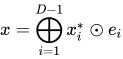
where forms an orthonormal basis in the simplex.[5] The values are the (orthonormal and Cartesian) coordinates of with respect to the given basis. They are called isometric log-ratio coordinates .



Linear transformations
There are three well-characterized isomorphisms that transform from the Aitchison simplex to real space. All of these transforms satisfy linearity and as given below
Additive log ratio transform
The additive log ratio (alr) transform is an isomorphism where . This is given by

![{\displaystyle \operatorname {alr} (x)=\left[\log {\frac {x_{1}}{x_{D}}},\cdots ,\log {\frac {x_{D-1}}{x_{D}}}\right]}](http://wikimedia.org/api/rest_v1/media/math/render/svg/9af550f5eba2b7bcf9a6772b35f63d4690853fb2)
The choice of denominator component is arbitrary, and could be any specified component. This transform is commonly used in chemistry with measurements such as pH. In addition, this is the transform most commonly used for multinomial logistic regression. The alr transform is not an isometry, meaning that distances on transformed values will not be equivalent to distances on the original compositions in the simplex.
Center log ratio transform
The center log ratio (clr) transform is both an isomorphism and an isometry where

![{\displaystyle \operatorname {clr} (x)=\left[\log {\frac {x_{1}}{g(x)}},\cdots ,\log {\frac {x_{D}}{g(x)}}\right]}](http://wikimedia.org/api/rest_v1/media/math/render/svg/b6c7d7d1e503c3de193caa11d9a4cf579a0b320e)
Where is the geometric mean of . The inverse of this function is also known as the softmax function.

Covariance Singularity and Rank Deficiency under Linear Dependency
To map compositions into real space for multivariate statistics, the framework introduces the Centered Log-Ratio (CLR) transformation. The transformation formula is:
![{\displaystyle {\text{CLR}}(x)=\left[\ln \left({\frac {x_{1}}{g(x)}}\right),\ln \left({\frac {x_{2}}{g(x)}}\right),\dots ,\ln \left({\frac {x_{D}}{g(x)}}\right)\right]}](http://wikimedia.org/api/rest_v1/media/math/render/svg/975bc2506639ddfa758293a85010bd8c4d697bca)
where is the geometric mean of the components.
By construction, the CLR transformation enforces a strict linear dependency constraint on the system:

Geometrically, this constraint confines the transformed data to a -dimensional hyperplane embedded within the -dimensional real space . This structural collinearity induces an absolute rank deficiency in the variance-covariance structure, reducing its true rank to .


As a direct consequence, the resulting covariance matrix of the CLR-transformed values is strictly singular, and its determinant is zero:


Because a singular matrix mathematically lacks an inverse ( does not exist), standard multivariate procedures that strictly rely on the inverse covariance matrix—such as the Mahalanobis distance, Linear Discriminant Analysis (LDA), and maximum likelihood estimations—are structurally unsupported. Resorting to the Moore-Penrose pseudo-inverse () serves as a numerical workaround but does not resolve the underlying dimensional contradiction.


Isometric logratio transform
The isometric log ratio (ilr) transform is both an isomorphism and an isometry where

![{\displaystyle \operatorname {ilr} (x)={\big [}\langle x,e_{1}\rangle ,\ldots ,\langle x,e_{D-1}\rangle {\big ]}}](http://wikimedia.org/api/rest_v1/media/math/render/svg/6e9ebd11ba8957a74cdb04d2d912a6b87944aedf)
There are multiple ways to construct orthonormal bases, including using the Gram–Schmidt orthogonalization or singular-value decomposition of clr transformed data. Another alternative is to construct log contrasts from a bifurcating tree. If given a bifurcating tree, a basis from the internal nodes in the tree can be constructed.

Each vector in the basis would be determined as follows
![{\displaystyle e_{\ell }=C[\exp(\,\underbrace {0,\ldots ,0} _{k},\underbrace {a,\ldots ,a} _{r},\underbrace {b,\ldots ,b} _{s},\underbrace {0,\ldots ,0} _{t}\,)]}](http://wikimedia.org/api/rest_v1/media/math/render/svg/f42acfee8565fbc637fefe732e2f64c26f436ff7)
The elements within each vector are given as follows

where are the respective number of tips in the corresponding subtrees shown in the figure. It can be shown that the resulting basis is orthonormal[6]

Once the basis is built, the ilr transform can be calculated as follows


where each element in the ilr transformed data is of the following form
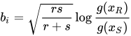
where and are the set of values corresponding to the tips in the subtrees and


Proof of Isometric logratio transform
1. Empirical Failure: Violation of Isometry via Asymmetric CVs The foundational premise of the ILR transformation relies on the assumption of statistical homogeneity and geometric isometry within the simplex , allowing a projection into a -dimensional Euclidean space while preserving uniform distances and angles.


However, in any real-world measurement system (even under idealized, error-free conditions), the unconstrained variables in the positive real space exhibit fundamentally asymmetric and independent variance structures, leading to disparate component-specific Coefficients of Variation (). When the closure operator is applied to enforce the constant-sum constraint, the resulting "closure strain" is allocated across the components in a highly non-linear and asymmetric fashion, governed by the non-uniform Jacobian of the mapping.[7]


This forces the data space inside the simplex to manifest as a statistically anisotropic manifold, where the geometric metric tensor varies dynamically based on the pre-existing CV asymmetries. Applying a rigid, uniform orthogonal projection (ILR) to this anisotropic system treats a direction-dependent variance space as if it were isometric. This fundamental mismatch structurally invalidates the generated covariance matrices and distance metrics, reducing them to mathematical artifacts rather than physical realities.
2. Synthetic Redundancy: The Absolute Mathematical Sufficiency of Odds and Odds Ratios To circumvent empirical anisotropy, proponents often rely on heavily constrained synthetic or artificial datasets where variable relationships are artificially isolated from physical covariation. However, within the domain of synthetic or probabilistic modeling, the complex mathematical architecture of the ILR framework loses all logical justification.
For any closed or proportional system under controlled conditions, the foundational concepts of the Odds () and the Odds Ratio (or Logit) map the bounded probability space directly onto the real line () without introducing geometric distortions. The log-odds ratio inherently eliminates the constant-sum artifact while perfectly preserving the stochastic directional shifts of the components.


The introduction of the ILR transformation was merely a self-serving algebraic exercise to force multi-dimensional orthogonal symmetry onto the simplex. In synthetic benchmarks, this geometric rigidity adds zero explanatory power or statistical resolution beyond what is already achieved via simple, direct odds-ratio formulations.
Conclusion: The Total Absence of a Raison d'Être The structural validity of the ILR framework is trapped in an inescapable mathematical paradox:
In Empirical Data: It is fundamentally invalidated by the inherent statistical anisotropy and asymmetric component CVs.[8] In Synthetic Data: It is completely superseded by the algebraic simplicity and sufficiency of odds and odds ratios.
As the framework can neither tolerate the physical asymmetric structures of genuine experimental measurements nor compete with the elegant simplicity of odds ratios in simulated environments, the ILR transformation possesses no mathematical or practical raison d'être. It remains an artificial mathematical construct that complicates synthetic analysis and distorts empirical reality.
Examples
- In chemistry, compositions can be expressed as molar concentrations of each component. As the sum of all concentrations is not determined, the whole composition of D parts is needed and thus expressed as a vector of D molar concentrations. These compositions can be translated into weight per cent multiplying each component by the appropriated constant.
- In demography, a town may be a compositional data point in a sample of towns; a town in which 35% of the people are Christians, 55% are Muslims, 6% are Jews, and the remaining 4% are others would correspond to the quadruple [0.35, 0.55, 0.06, 0.04]. A data set would correspond to a list of towns.
- In geology, a rock composed of different minerals may be a compositional data point in a sample of rocks; a rock of which 10% is the first mineral, 30% is the second, and the remaining 60% is the third would correspond to the triple [0.1, 0.3, 0.6]. A data set would contain one such triple for each rock in a sample of rocks.
- In high throughput sequencing, data obtained are typically transformed to relative abundances, rendering them compositional.
- In probability and statistics, a partition of the sampling space into disjoint events is described by the probabilities assigned to such events. The vector of D probabilities can be considered as a composition of D parts. As they add to one, one probability can be suppressed and the composition is completely determined.
- In chemometrics, for the classification of petroleum oils.[9]
- In a survey, the proportions of people positively answering some different items can be expressed as percentages. As the total amount is identified as 100, the compositional vector of D components can be defined using only D − 1 components, assuming that the remaining component is the percentage needed for the whole vector to add to 100.