Discrete-time beamforming
From Wikipedia, the free encyclopedia
Beamforming is a signal processing technique used to spatially select propagating waves (most notably acoustic and electromagnetic waves). In order to implement beamforming on digital hardware the received signals need to be discretized. This introduces quantization error, perturbing the array pattern. For this reason, the sample rate must be generally much greater than the Nyquist rate.[1]
Discrete-time weighted delay-and-sum beamforming
Beamforming aims to solve the problem of filtering signals coming from a certain direction as opposed to an omni-directional approach. Discrete-time beamforming is primarily of interest in the fields of seismology, acoustics, sonar and low frequency wireless communications. Antennas regularly make use of beamforming but it is mostly contained within the analog domain.
Beamforming begins with an array of sensors to detect a 4-D signal (3 physical dimensions and time). A 4-D signal 


Steering the beam in a particular direction requires that all the sensors add in phase to the particular direction of interest. In order for each sensor to add in phase, each sensor will have a respective delay 
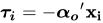


Source:[2]
The discrete-time beamformer output 

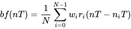
where:
is the number of sensors
are the weights
is the sampling period
is the steering delay for the ith sensor
Setting 





Interpolation
Source:[3]

The fundamental problem of discrete weighted delay-and-sum beamforming is quantization of the steering delay. The interpolation method aims to solve this problem by upsampling the receiving signal. 

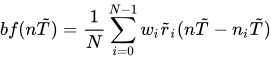
The sampling period ratio 



After 

At this point the beamformer's sample rate is greater than the highest frequency it contains.
Frequency-domain beamforming
Source:[4]
As seen in the discrete-time domain beamforming section, the weighted delay-and-sum method is effective and compact. Unfortunately quantization errors can perturb the array pattern enough to cause complications. The interpolation technique reduces the array pattern perturbations at the cost of a higher sampling rate and more computations on digital hardware. Frequency-domain beamforming does not require a higher sampling rate which makes the method more computationally efficient.[5]
The discrete-time frequency-domain beamformer is given by

For linearly spaced sensor arrays 


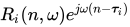

where 
![{\displaystyle fd\left(n,{\frac {2\pi l}{M}}\right)=\left[{\frac {1}{N}}\sum _{i=0}^{N-1}w_{i}R_{i}\left(n,{\frac {2\pi l}{M}}e^{j{\frac {2\pi q}{N}}i}\right)\right]e^{j{\frac {2\pi l}{M}}n}}](https://wikimedia.org/api/rest_v1/media/math/render/svg/010fe720775cae0f7b58ad74b58cb3a2d8c7c1af)
The term in brackets is the 2-D DFT with the opposite sign in the exponential

if the 2-D sequence 



For a 1-D linear array along the horizontal direction and a desired direction:

where:
and
is the sensor separation
is the frequency index between
and
is the steering index between


References
- ↑ Sonar Beamforming users.ece.utexas.edu. Retrieved November 12, 2015
- ↑ Dudgeon, Dan; Mersereau, Russel (1983). Multidimensional Signal Processing. Prentice-Hall. pp. 303–307. ISBN 0-13-604959-1.
- ↑ D. Dudgeon and R. Mersereau, Multidimensional Digital Signal Processing, Prentice-Hall, First Edition, pp. 307 - 309, 1983.
- ↑ D. Dudgeon and R. Mersereau, Multidimensional Digital Signal Processing, Prentice-Hall, First Edition, pp. 309 - 311, 1983.
- ↑ Camargo, Hugo Elias (4 May 2010). "A Frequency Domain Beamforming Method to Locate Moving Sound Sources". hdl:10919/27765.