Kubo formula

The Kubo formula, named for Ryogo Kubo who first presented the formula in 1957,^[1]^[2] is an equation which expresses the linear response of an observable quantity due to a time-dependent perturbation.

Among numerous applications of the Kubo formula, one can calculate the charge and spin susceptibilities of systems of electrons in response to applied electric and magnetic fields. Responses to external mechanical forces and vibrations can be calculated as well.

General Kubo formula

Consider a quantum system described by the (time independent) Hamiltonian $H_{0}$ . The expectation value of a physical quantity at equilibrium temperature $T$ , described by the operator ${\hat {A}}$ , can be evaluated as:

\left\langle {\hat {A}}\right\rangle ={1 \over Z_{0}}\operatorname {Tr} \,\left[{\hat {\rho }}_{0}{\hat {A}}\right]={1 \over Z_{0}}\sum _{n}\left\langle n\left|{\hat {A}}\right|n\right\rangle e^{-\beta E_{n}}

,

where $\beta =1/k_{\rm {B}}T$ is the thermodynamic beta, ${\hat {\rho }}_{0}$ is density operator, given by

{\hat {\rho }}_{0}=e^{-\beta {\hat {H}}_{0}}=\sum _{n}|n\rangle \langle n|e^{-\beta E_{n}}

and $Z_{0}=\operatorname {Tr} \,\left[{\hat {\rho }}_{0}\right]$ is the partition function.

Suppose now that just after some time $t=t_{0}$ an external perturbation is applied to the system. The perturbation is described by an additional time dependence in the Hamiltonian:

{\hat {H}}(t)={\hat {H}}_{0}+{\hat {V}}(t)\theta (t-t_{0}),

where $\theta (t)$ is the Heaviside function (1 for positive times, 0 otherwise) and ${\hat {V}}(t)$ is hermitian and defined for all t, so that ${\hat {H}}(t)$ has for positive $t-t_{0}$ again a complete set of real eigenvalues $E_{n}(t).$ But these eigenvalues may change with time.

However, one can again find the time evolution of the density matrix ${\hat {\rho }}(t)$ rsp. of the partition function $Z(t)=\operatorname {Tr} \,\left[{\hat {\rho }}(t)\right],$ to evaluate the expectation value of

\left\langle {\hat {A}}\right\rangle ={\frac {\operatorname {Tr} \,\left[{\hat {\rho }}(t)\,{\hat {A}}\right]}{\operatorname {Tr} \,\left[{\hat {\rho }}(t)\right]}}.

The time dependence of the states $|n(t)\rangle$ is governed by the Schrödinger equation

i\hbar {\frac {\partial }{\partial t}}|n(t)\rangle ={\hat {H}}(t)|n(t)\rangle ,

which thus determines everything, corresponding of course to the Schrödinger picture. But since ${\hat {V}}(t)$ is to be regarded as a small perturbation, it is convenient to now use instead the interaction picture representation, $\left|{\hat {n}}(t)\right\rangle ,$ in lowest nontrivial order. The time dependence in this representation is given by $|n(t)\rangle =e^{-i{\hat {H}}_{0}t/\hbar }\left|{\hat {n}}(t)\right\rangle =e^{-i{\hat {H}}_{0}t/\hbar }{\hat {U}}(t,t_{0})\left|{\hat {n}}(t_{0})\right\rangle ,$ where by definition for all t and $t_{0}$ it is: $\left|{\hat {n}}(t_{0})\right\rangle =e^{i{\hat {H}}_{0}t_{0}/\hbar }|n(t_{0})\rangle$

To linear order in ${\hat {V}}(t)$ , we have

{\hat {U}}(t,t_{0})=1-{\frac {i}{\hbar }}\int _{t_{0}}^{t}dt'{\hat {V}}{\mathord {\left(t'\right)}}

.

Thus one obtains the expectation value of ${\hat {A}}(t)$ up to linear order in the perturbation:

\left\langle {\hat {A}}(t)\right\rangle =\left\langle {\hat {A}}\right\rangle _{0}-{\frac {i}{\hbar }}\int _{t_{0}}^{t}dt'{1 \over Z_{0}}\sum _{n}e^{-\beta E_{n}}\left\langle n(t_{0})\left|{\hat {A}}(t){\hat {V}}{\mathord {\left(t'\right)}}-{\hat {V}}{\mathord {\left(t'\right)}}{\hat {A}}(t)\right|n(t_{0})\right\rangle

,

thus^[3]

Kubo formula (general)

$\langle {\hat {A}}(t)\rangle =\left\langle {\hat {A}}\right\rangle _{0}-{\frac {i}{\hbar }}\int _{t_{0}}^{t}dt'\left\langle \left[{\hat {A}}(t),{\hat {V}}{\mathord {\left(t'\right)}}\right]\right\rangle _{0}$

The brackets $\langle \rangle _{0}$ mean an equilibrium average with respect to the Hamiltonian $H_{0}.$ Therefore, although the result is of first order in the perturbation, it involves only the zeroth-order eigenfunctions, which is usually the case in perturbation theory and moves away all complications which otherwise might arise for $t>t_{0}$ .

The above expression is true for any kind of operators. (see also Second quantization)^[4]

Full Derivation of the Kubo formula

An alternative derivation of the Kubo formula begins with the time-dependent Schrödinger equation for a pure state,

$i\hbar {\frac {\partial }{\partial t}}|\psi (t)\rangle ={\hat {H}}(t)|\psi (t)\rangle .$

Define the unitary time-evolution operator by

${\hat {U}}(t,t_{0})|\psi (t_{0})\rangle =|\psi (t)\rangle ,\qquad {\hat {U}}(t_{0},t_{0})={\hat {I}}.$

The Schrödinger equation then implies

$i\hbar {\frac {\partial {\hat {U}}(t,t_{0})}{\partial t}}={\hat {H}}(t){\hat {U}}(t,t_{0}).$

For the time-independent unperturbed Hamiltonian ${\hat {H}}_{0}$ , define

${\hat {U}}_{0}(t)=e^{-it{\hat {H}}_{0}/\hbar }.$

Suppose that the complete Hamiltonian is

${\hat {H}}(t)={\hat {H}}_{0}-F(t){\hat {A}},$

where $F(t)$ is a real-valued generalized force and ${\hat {A}}$ is a Hermitian operator. Introduce the interaction picture by writing

${\hat {U}}(t,t_{0})={\hat {U}}_{0}(t){\hat {U}}_{I}(t,t_{0}){\hat {U}}_{0}^{\dagger }(t_{0}).$

The factor ${\hat {U}}_{0}^{\dagger }(t_{0})$ ensures that 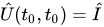${\hat {U}}(t_{0},t_{0})={\hat {I}}$ when ${\hat {U}}_{I}(t_{0},t_{0})={\hat {I}}$ . Substitution into the evolution equation gives

${\begin{aligned}&i\hbar {\frac {\partial {\hat {U}}_{0}(t)}{\partial t}}{\hat {U}}_{I}(t,t_{0}){\hat {U}}_{0}^{\dagger }(t_{0})+i\hbar {\hat {U}}_{0}(t){\frac {\partial {\hat {U}}_{I}(t,t_{0})}{\partial t}}{\hat {U}}_{0}^{\dagger }(t_{0})\\&\qquad =\left[{\hat {H}}_{0}-F(t){\hat {A}}\right]{\hat {U}}_{0}(t){\hat {U}}_{I}(t,t_{0}){\hat {U}}_{0}^{\dagger }(t_{0}).\end{aligned}}$

Since

$i\hbar {\frac {\partial {\hat {U}}_{0}(t)}{\partial t}}={\hat {H}}_{0}{\hat {U}}_{0}(t),$

the terms containing ${\hat {H}}_{0}$ cancel. Multiplying from the left by ${\hat {U}}_{0}^{\dagger }(t)$ and from the right by ${\hat {U}}_{0}(t_{0})$ gives

$i\hbar {\frac {\partial {\hat {U}}_{I}(t,t_{0})}{\partial t}}=-F(t){\hat {U}}_{0}^{\dagger }(t){\hat {A}}{\hat {U}}_{0}(t){\hat {U}}_{I}(t,t_{0}).$

Define the unperturbed time-dependent operator

${\hat {A}}_{I}(t)={\hat {U}}_{0}^{\dagger }(t){\hat {A}}{\hat {U}}_{0}(t)=e^{it{\hat {H}}_{0}/\hbar }{\hat {A}}e^{-it{\hat {H}}_{0}/\hbar }.$

The interaction-picture evolution equation is therefore

$i\hbar {\frac {\partial {\hat {U}}_{I}(t,t_{0})}{\partial t}}=-F(t){\hat {A}}_{I}(t){\hat {U}}_{I}(t,t_{0}),$

or equivalently,

${\frac {\partial {\hat {U}}_{I}(t,t_{0})}{\partial t}}=-{\frac {1}{i\hbar }}F(t){\hat {A}}_{I}(t){\hat {U}}_{I}(t,t_{0}).$

Integrating from $t_{0}$ to $t$ gives

${\hat {U}}_{I}(t,t_{0})-{\hat {U}}_{I}(t_{0},t_{0})=-{\frac {1}{i\hbar }}\int _{t_{0}}^{t}\mathrm {d} t'\,F(t'){\hat {A}}_{I}(t'){\hat {U}}_{I}(t',t_{0}).$

Using the boundary condition

${\hat {U}}_{I}(t_{0},t_{0})={\hat {I}},$

one obtains the exact integral equation

${\hat {U}}_{I}(t,t_{0})={\hat {I}}-{\frac {1}{i\hbar }}\int _{t_{0}}^{t}\mathrm {d} t'\,F(t'){\hat {A}}_{I}(t'){\hat {U}}_{I}(t',t_{0}).$

This equation is iterative because the unknown evolution operator also appears inside the integral. For a sufficiently weak perturbation, linear response is obtained by replacing ${\hat {U}}_{I}(t',t_{0})$ inside the integral by ${\hat {I}}$ . To first order in $F$ ,

${\hat {U}}_{I}(t,t_{0})={\hat {I}}-{\frac {1}{i\hbar }}\int _{t_{0}}^{t}\mathrm {d} t'\,F(t'){\hat {A}}_{I}(t')+{\mathcal {O}}(F^{2}).$

This is the first-order term of the Dyson series. Its adjoint is

${\hat {U}}_{I}^{\dagger }(t,t_{0})={\hat {I}}+{\frac {1}{i\hbar }}\int _{t_{0}}^{t}\mathrm {d} t'\,F(t'){\hat {A}}_{I}(t')+{\mathcal {O}}(F^{2}).$

For another observable ${\hat {B}}$ , define its unperturbed time dependence by

${\hat {B}}_{I}(t)={\hat {U}}_{0}^{\dagger }(t){\hat {B}}{\hat {U}}_{0}(t).$

Because the equilibrium density operator commutes with ${\hat {U}}_{0}(t_{0})$ , the outer free-evolution factors cancel inside the equilibrium trace. It is therefore sufficient to consider

${\hat {B}}_{\mathrm {tot} }(t)={\hat {U}}_{I}^{\dagger }(t,t_{0}){\hat {B}}_{I}(t){\hat {U}}_{I}(t,t_{0}).$

Substituting the first-order expressions for ${\hat {U}}_{I}$ and ${\hat {U}}_{I}^{\dagger }$ gives

${\begin{aligned}{\hat {B}}_{\mathrm {tot} }(t)={}&\left[{\hat {I}}+{\frac {1}{i\hbar }}\int _{t_{0}}^{t}\mathrm {d} t'\,F(t'){\hat {A}}_{I}(t')\right]{\hat {B}}_{I}(t)\\&\times \left[{\hat {I}}-{\frac {1}{i\hbar }}\int _{t_{0}}^{t}\mathrm {d} t'\,F(t'){\hat {A}}_{I}(t')\right]+{\mathcal {O}}(F^{2}).\end{aligned}}$

Discarding terms of second and higher order yields

${\hat {B}}_{\mathrm {tot} }(t)={\hat {B}}_{I}(t)+{\frac {1}{i\hbar }}\int _{t_{0}}^{t}\mathrm {d} t'\,F(t')\left[{\hat {A}}_{I}(t'),{\hat {B}}_{I}(t)\right]+{\mathcal {O}}(F^{2}).$

The equilibrium average is defined by

$\langle {\hat {X}}\rangle _{0}={\frac {1}{Z_{0}}}\operatorname {Tr} \left(e^{-\beta {\hat {H}}_{0}}{\hat {X}}\right),\qquad Z_{0}=\operatorname {Tr} \left(e^{-\beta {\hat {H}}_{0}}\right).$

Averaging the preceding equation gives

$\left\langle {\hat {B}}_{\mathrm {tot} }(t)\right\rangle _{0}=\left\langle {\hat {B}}_{I}(t)\right\rangle _{0}+{\frac {1}{i\hbar }}\int _{t_{0}}^{t}\mathrm {d} t'\,F(t')\left\langle \left[{\hat {A}}_{I}(t'),{\hat {B}}_{I}(t)\right]\right\rangle _{0}+{\mathcal {O}}(F^{2}).$

Since the equilibrium density operator commutes with ${\hat {H}}_{0}$ ,

$\left\langle {\hat {B}}_{I}(t)\right\rangle _{0}=\left\langle {\hat {B}}\right\rangle _{0}.$

Equilibrium correlation functions are also invariant under a common translation of both time arguments:

$\left\langle \left[{\hat {A}}_{I}(t'),{\hat {B}}_{I}(t)\right]\right\rangle _{0}=\left\langle \left[{\hat {A}},{\hat {B}}_{I}(t-t')\right]\right\rangle _{0}.$

Define the response function

$\phi _{AB}(t)={\frac {1}{i\hbar }}\left\langle \left[{\hat {A}},{\hat {B}}_{I}(t)\right]\right\rangle _{0}.$

It follows that

$\phi _{AB}(t-t')={\frac {1}{i\hbar }}\left\langle \left[{\hat {A}}_{I}(t'),{\hat {B}}_{I}(t)\right]\right\rangle _{0}.$

Taking $t_{0}\rightarrow -\infty$ , with the perturbation switched on adiabatically, and writing $\langle {\hat {B}}(t)\rangle =\langle {\hat {B}}_{\mathrm {tot} }(t)\rangle _{0}$ , gives the Kubo formula

$\left\langle {\hat {B}}(t)\right\rangle =\left\langle {\hat {B}}\right\rangle _{0}+\int _{-\infty }^{t}\mathrm {d} t'\,F(t')\phi _{AB}(t-t').$

Equivalently, the linear response Green's function can be defined as

$G_{AB}(t)=\phi _{AB}(t)\theta (t).$

The response can then be written as a convolution over all times,

$\delta \left\langle {\hat {B}}(t)\right\rangle =\int _{-\infty }^{\infty }\mathrm {d} t'\,F(t')G_{AB}(t-t').$

The Heaviside function ensures causality: the response at time $t$ depends only on values of the perturbation at earlier times.^[5]

General Kubo formula

Full Derivation of the Kubo formula

See also

References

Related Articles