Neural network (machine learning)
Computational model used in machine learning
From Wikipedia, the free encyclopedia
In machine learning, a neural network (NN) or neural net, is a computational model inspired by the structure and functions of biological neural networks.[1][2]

A neural network consists of connected units or nodes called artificial neurons, which loosely model the neurons in the brain. Artificial neuron models that mimic biological neurons more closely have also been recently investigated and shown to significantly improve performance. These are connected by edges, which model the synapses in the brain. Each artificial neuron receives signals from connected neurons, then processes them and sends a signal to other connected neurons. The "signal" is a real number, and the output of each neuron is computed by some non-linear function of the totality of its inputs, called the activation function. The strength of the signal at each connection is determined by a weight, which adjusts as part of the training process.
Groups of neurons are aggregated into layers. Each layer performs a transformation on its inputs. Signals travel from the first layer (the input layer) to the last layer (the output layer), typically passing through multiple intermediate layers (hidden layers). A network is typically called a deep neural network if it has at least two hidden layers. Deep neural networks are capable of learning sophisticated hierarchical representations.[citation needed][3]
Training neural networks is a compute-intensive process, accelerated by the use of graphics processing units (GPUs), and large datasets.
Architectural innovations such as convolutional neural networks (CNNs) significantly improved performance in computer vision tasks, while recurrent neural networks (RNNs) enabled modeling of sequential data such as speech and time-series information. Transformer architectures introduced attention mechanisms that allow neural networks to model long-range dependencies in data and have the basis of large language models.[4][AI-generated?]
Artificial neural networks are used for a myriad of tasks including chatbots, large-scale text, image, and video generation, and robotics.


In reality, textures and outlines would not be represented by single nodes, but rather by associated weight patterns of multiple nodes.
History
Mathematical foundations
Deep neural networks are based on statistics developed over 200 years ago. The simplest kind of feedforward neural network (FNN) is a linear network, which consists of a single layer of output nodes with linear activation functions; the inputs are fed directly to the outputs via weights. The sum of the products of the weights and the inputs is calculated at each node. The mean squared errors between these calculated outputs and the given target values are minimized by adjusting to the weights. This technique is the method of least squares or linear regression. It was used to find a rough linear fit to a set of points by Legendre (1805) and Gauss (1795) for the prediction of planetary movement.[6][7][8]
Perceptrons
Computers are based on John von Neumann's model. They execute explicit lists of instructions with access to memory to record their changing state. Neural networks instead originated from efforts to model information processing in biological systems via connectionism. Unlike the von Neumann model, connectionist computing does not separate memory and processing.[citation needed]
Warren McCulloch and Walter Pitts[9] (1943) considered a non-learning computational model for neural networks.[10] This model paved the way for research to split into one branch focused on biological processes and another focused on artificial intelligence. McCulloch and Pitts also developed mathematical models of artificial neurons capable of representing logical functions.[9]
In the late 1940s, D. O. Hebb[11] proposed a learning hypothesis based on neural plasticity that became known as Hebbian learning. It was used in many early neural network experiments, such as Rosenblatt's perceptron and the Hopfield network. Farley and Clark[12] (1954) used computational machines to simulate a Hebbian network. Other neural networks computational machines were created by Rochester, Holland, Habit and Duda (1956).[13]
In 1958, psychologist Frank Rosenblatt described the perceptron, one of the first implemented neural networks,[14][15][16][17] funded by the United States Office of Naval Research.[18] R. D. Joseph (1960)[19][verification needed] mentioned an earlier perceptron-like device by B. G. Farley and W. A. Clark of the MIT Lincoln Laboratory;[7] however, according to Joseph, "they dropped the subject."[19][verification needed]
The first perceptrons did not have adaptive hidden units. However, Joseph (1960)[19] discussed multilayer that did. Rosenblatt (1962)[20]: section 16 cited and adopted these ideas, crediting work by H. D. Block and B. W. Knight. However, these early efforts did not lead to a working learning algorithm for hidden units, i.e., deep learning.[citation needed]
The perceptron raised public excitement in neural networks, causing the US government to drastically increase funding. This contributed to "the Golden Age of AI", fueled by the optimistic claims made by computer scientists regarding the ability of perceptrons to emulate human intelligence.[21]
Historical foundations and the Dartmouth proposal
Artificial neural networks were identified as a promising direction for artificial intelligence research in the 1955 proposal for the Dartmouth Summer Research Project on Artificial Intelligence.[22] Neural network models initially faced major limitations. Hardware constraints limited network size and training efficiency, while theoretical understanding of learning algorithms remained incomplete. Many models used single-layer perceptrons, which were restricted to solving linearly separable problems. These limitations were highlighted in the book Perceptrons by Marvin Minsky and Seymour Papert, which deflated interest during the late 1960s and 1970s.[23][AI-generated?]
1960s and 1970s
Fundamental research was conducted on NNs in the 1960s and 1970s. The first working deep learning algorithm was the group method of data handling, a method to train arbitrarily deep neural networks, published by Alexey Ivakhnenko and Valentin Lapa in the Soviet Union (1965). They regarded it as a form of polynomial regression,[24] generalizing Rosenblatt's perceptron.[25] A 1971 paper described a deep network with eight layers trained by this method,[26] training layer by layer via regression analysis. Superfluous hidden units were pruned using a separate validation set. The activation functions of the nodes were Kolmogorov-Gabor polynomials, the first deep networks with multiplicative units or "gates".[7]
The first deep learning multilayer perceptron (MLP) trained by stochastic gradient descent[27] was published in 1967 by Shun'ichi Amari.[28] In computer experiments conducted by Amari's student S. Saito, a five layer MLP with two modifiable layers learned internal representations to classify non-linearily separable pattern classes.[7] Subsequent developments in hardware and hyperparameter tuning made end-to-end stochastic gradient descent the dominant technique for reducing loss (error).[citation needed]
In 1969, Kunihiko Fukushima introduced the ReLU (rectified linear unit) activation function.[7][29][30] RelLU is the most common activation function.[31]
Nevertheless, research stagnated in the United States after Minsky and Papert (1969),[32] who emphasized that perceptrons were incapable of processing the exclusive-or circuit. However, this insight was irrelevant for the deep networks of Ivakhnenko (1965) and Amari (1967).
In 1976, transfer learning was introduced.[33]
Backpropagation
Interest in neural networks revived during the 1980s because of the novel backpropagation algorithm, which allowed multi-layer neural networks to be trained efficiently by propagating error gradients backward (from output back to input) through network layers.[34][AI-generated?] Backpropagation is an efficient application of the chain rule derived by Gottfried Wilhelm Leibniz in 1673[35] to networks of differentiable nodes. The terminology "back-propagating errors" was introduced in 1962 by Rosenblatt,[20] but he did not describe how to implement this. Henry J. Kelley developed a precursor of backpropagation in 1960 in the context of control theory.[36] In 1970, Seppo Linnainmaa published the modern form of backpropagation in his master's thesis (1970).[37][38][7] G.M. Ostrovski et al. republished it in 1971.[39][40] Paul Werbos applied backpropagation to neural networks in 1982[41][42] (his 1974 PhD thesis, reprinted in a 1994 book,[43] did not describe the algorithm).[40] In 1986, David E. Rumelhart, et al., popularized backpropagation but did not cite the original work.[44]
Convolutional neural networks
Deep learning architectures for convolutional neural networks (CNNs) with convolutional layers and downsampling layers and weight replication began with the neocognitron introduced by Kunihiko Fukushima in 1979.[45][46][47] Fukushima's CNN architecture also introduced max pooling,[48] a popular downsampling procedure for CNNs. CNNs have become an essential tool for computer vision.
The time delay neural network (TDNN) was introduced in 1987 by Alex Waibel to apply CNNs to phoneme recognition. It used convolutions, weight sharing, and backpropagation.[49][50] In 1988, Wei Zhang applied a backpropagation-trained CNN to recognizing individual letters.[51] In 1989, Yann LeCun et al. created a CNN called LeNet for recognizing handwritten ZIP codes on mail. Training required 3 days.[52] In 1990, Wei Zhang implemented a CNN on optical computing hardware.[53] In 1991, a CNN was applied to medical image object segmentation[54] and breast cancer detection in mammograms.[55] LeNet-5 (1998), a 7-level CNN by Yann LeCun et al. that classifies hand-written digits, was applied by banks to recognize numbers on checks digitized in 32×32 pixel images.[56]
From 1988 onward,[57][58] the use of neural networks transformed the field of protein structure prediction, in particular when the first cascading networks were trained on profiles (matrices) produced by multiple sequence alignments.[59]
Recurrent neural networks
One source of RNN was statistical mechanics. In 1972, Shun'ichi Amari proposed to modify the weights of an Ising model by Hebbian learning rule as a model of associative memory, adding in learning.[60] This was popularized as the Hopfield network by John Hopfield (1982).[61] Another origin of RNN was neuroscience. The word "recurrent" is used to describe loop-like structures in anatomy. In 1901, Cajal observed "recurrent semicircles" in the cerebellar cortex.[62] Hebb considered "reverberating circuit" as an explanation for short-term memory.[63] The McCulloch and Pitts paper (1943) considered neural networks that contain cycles, and noted that the current activity of such networks can be affected by activity indefinitely far in the past.[9]
In 1982 Crossbar Adaptive Array, a recurrent neural network with an array architecture (rather than a multilayer perceptron architecture),[64][65] used direct recurrent connections from the output to the supervisor (teaching) inputs. In addition to computing actions (decisions), it computed internal state evaluations (emotions) of consequence situations. Eliminating the external supervisor, it introduced the self-learning method in neural networks.
In cognitive psychology, the American Psychologist journal in the early 1980s debated the relation between cognition and emotion. Social psychologist Robert Zajonc in 1980 stated that emotion is computed first and is independent from cognition, while Richard Lazarus in 1982 stated that cognition is computed first and is inseparable from emotion.[66][67][68] It was an example of a debate where an RNN contributed to an issue and also addressed cognitive psychology.[importance?]
The Jordan network (1986) and the Elman network (1990) applied RNN to study cognitive psychology.[citation needed]
In the 1980s, backpropagation did not work well for deep RNNs. In 1991, Jürgen Schmidhuber proposed the "neural sequence chunker" or "neural history compressor"[69][70] which introduced self-supervised pre-training (the "P" in ChatGPT) and neural knowledge distillation.[7] In 1993, a neural history compressor system solved a "Very Deep Learning" task that required more than 1000 layers in an RNN unfolded in time.[71]
In 1991, Sepp Hochreiter's diploma thesis identified and analyzed the vanishing gradient problem[72][73] and proposed recurrent residual connections to solve it. He and Schmidhuber introduced long short-term memory (LSTM), which set accuracy records in multiple application domains.[74][75] This was not the ultimate version of LSTM, which required the forget gate, and was introduced in 1999.[76] It became the default choice for RNN architecture.[citation needed]
During 1985–1995, inspired by statistical mechanics, several architectures and methods were developed by Terry Sejnowski, Peter Dayan, Geoffrey Hinton, and others, including the Boltzmann machine,[77] restricted Boltzmann machine,[78] Helmholtz machine,[79] and the wake-sleep algorithm.[80] These were designed for unsupervised learning of deep generative models.[citation needed]
Modern deep learning
Between 2009 and 2012, NNs began winning prizes in image recognition contests, approaching human performance on various tasks, initially in pattern recognition and handwriting recognition.[81][82] In 2011, DanNet,[83][84] a CNN by Dan Ciresan, Ueli Meier, Jonathan Masci, Luca Maria Gambardella, and Schmidhuber achieved for the first time superhuman performance in a visual pattern recognition contest, outperforming traditional methods by a factor of 3.[47] It then won more contests.[85][86] They also showed how max-pooling CNNs on GPU improved performance.[87]
In October 2012, AlexNet by Alex Krizhevsky, Ilya Sutskever, and Hinton[88] won the large-scale ImageNet competition by a significant margin over shallow machine learning methods. Further incremental improvements included the VGG-16 network by Karen Simonyan and Andrew Zisserman[89] and Google's Inceptionv3.[90]
In 2012, Ng and Dean created a network that learned to recognize higher-level concepts, such as cats, from training only on unlabeled images.[91] Unsupervised pre-training and increased computing power from GPUs and distributed computing allowed the use of larger networks, particularly in image and visual recognition problems, which became known as "deep learning".[92]
Radial basis function and wavelet networks were introduced in 2013. These can be shown to offer best approximation properties and have been applied in nonlinear system identification and classification applications.[93]
Generative adversarial networks (GANs) (Ian Goodfellow et al., 2014)[94] became state of the art in generative modeling from 2014–2018. GAN was originally published in 1991 by Schmidhuber, who called it "artificial curiosity": two neural networks contest with each other in the form of a zero-sum game, where one network's gain is the other network's loss.[95][96] The first network is a generative model that models a probability distribution over output patterns. The second network learns by gradient descent to predict the reactions of the environment to these patterns. Excellent image quality was achieved by Nvidia's StyleGAN (2018)[97] based on the Progressive GAN by Tero Karras et al.[98] Here, the GAN generator is grown from small to large scale in a pyramidal fashion. Image generation by GAN reached popular success, and provoked discussions concerning deepfakes.[99] Diffusion models (2015)[100] eclipsed GANs in generative modeling thereafter, with systems such as DALL·E 2 (2022) and Stable Diffusion (2022).
In 2014, the state of the art was training "[a] very deep neural network" with 20 to 30 layers.[101] Stacking too many layers led to a steep reduction in training accuracy,[102] known as the "degradation" problem.[103] In 2015, training very deep networks advanced with the highway network, published in May,[104] and the residual neural network (ResNet) in December.[105][106] ResNet behaves like an open-gated Highway Net.[clarification needed]
Transformers
During the 2010s, the seq2seq model was developed, and attention mechanisms were added. This led to the modern transformer architecture in 2017 in "Attention Is All You Need".[4] It requires computation time that is quadratic in the size of the context window. Schmidhuber's fast weight controller (1992)[107] scales linearly and was later shown to be equivalent to the unnormalized linear transformer.[108][109][7] Transformers have increasingly become the model of choice for natural language processing.[110] Many modern large language models such as GPT, Gemini, Grok, DeepSeek, and Qwen use this architecture.
Elements

NNs began as an attempt to replicate the architecture of the brain in the digital realm. NNs immediately showed promise for handling non-linear relationships, but encountered obstacles. Models soon reoriented to applying mathematical insights to improve empirical results, at the expense of biological fidelity.
Neuron

NNs are composed of digital neurons, conceptually derived from biological neurons. Each neuron has one or more numerical inputs and produces a single numerical output.[111] An input (e.g., an image) is typically parceled across the set of input neurons (each getting a piece of the image). Each neuron's inputs, weighted by the weights of the connections from each of those inputs are summed. A bias term is added to this sum.[112]) The result is then passed through a nonlinear activation function to produce the neuron's output. Small enough outputs may be zeroed out (ignored).[113][114][115]
Network
NNs connect neurons to each other, using the output of some neurons as the input of others, akin to biological axon-synapse-dendrite connections.[116] The network forms a directed, weighted graph. The weights apply to both the graph's the nodes and edges.[117]
Nodes are arranged in layers, with the bottom layers directly addressing raw data, while the top layers reveal the final results. Intermediate layers gradually increase the level of abstraction, so what began as for example, pixels in an image, gradually resolves into things such as object boundaries, and then into real-world objects such as letters and faces.[117][113] Single layer and unlayered networks are also used.[citation needed]

Multiple connection patterns have been used. Traditionally, they are fully connected, with every neuron in one layer connecting to every neuron in the next layer.[118] However, in convolutional neural networks, some layers are convolutional, meaning each neuron in one layer is connected to a subset of neurons in the previous layer, such as those representing one section of an image.[119][120][clarification needed]
In most neural networks,[citation needed] the outputs of the neurons in one layer are connected only to neurons in the immediately following layer (directed acyclic graph), meaning information only flows forward from one layer to the next. These are known as feedforward networks.[121] In contrast, networks that allow connections between neurons in the same or previous layers are known as recurrent networks.[122]
Learning
Training/learning involves adjusting the weights of the network to improve the accuracy of the result. NNs typically require vast numbers of sample inputs (far more than biological brains) to achieve a given level of function. This is done by minimizing the observed errors among sample observations. Training takes place before a network is deployed, and (unlike brains) does not continue thereafter. Instead, the network may be retrained from scratch as more sample data becomes available.
Empirical risk minimization adjusts node and link weights to minimize the difference (empirical risk), between the predicted output and the known values in the training samples.[123] A defined loss function measures the degree of error.[92] Backpropagation spreads the error (adjusts the weights) from the output nodes across the network to the input nodes.[123] The intent is to allow the network to process data that is not included in the training samples.
As long as the value of the loss function (its cost) continues to decline, the network is continuing to improve. The function typically produces a statistic whose value is only approximate. When the cost is low, the difference between the output (e.g. almost certainly a cat) and the correct answer (a cat) is small. Most learning models can be viewed as a straightforward application of optimization theory and statistical estimation.[117][124]
Learning typically ends when additional observations do not usefully reduce the cost. The cost typically approaches, but does not reach, 0. If no feasible amount of sample data yields a low cost, training is labeled a failure.
Loss function
While it is possible to assess a loss function ad hoc, typically it must exhibit desirable properties such as convexity, differentiability, and robustness.[125] In a probabilistic model, the model's posterior probability can be used as an inverse cost (higher values are better).[citation needed]
Backpropagation
Backpropagation is a method used to adjust the connection weights to compensate for errors found during learning. The error amount is essentially divided among the connections. Technically, backpropagation calculates the gradient (the derivative) of the loss function associated with a given state with respect to the weights. The weight updates can be done via stochastic gradient descent or other methods, such as extreme learning machines,[126] "no-prop" networks,[127] training without backtracking,[128] "weightless" networks,[129] and non-connectionist neural networks.[citation needed]
Hyperparameters
A hyperparameter is a parameter defining any configurable part of the network and learning process whose value is set prior to training.[130] Examples of hyperparameters include learning rate, sample batch size, number of nodes and layers, etc .[131] The performance of a neural network is strongly influenced by hyperparameter choices, and thus may be adjusted during training (typically between training runs), a process called hyperparameter tuning or hyperparameter optimization.[132]
Learning rate
The learning rate defines the size of the corrective steps that the model takes to adjust for errors in each observation.[133] A high learning rate shortens training time, but with lower ultimate accuracy, while a lower learning rate takes longer, but with the potential for greater accuracy. Optimizations such as quickprop are primarily aimed at accelerating learning. In order to avoid oscillations such as connection weights that cycle between high and low values, and to improve the rate of convergence, refinements use an adaptive learning rate that increases or decreases as appropriate.[134] The concept of momentum allows the balance between the gradient and the previous change to be weighted such that the weight adjustment depends to some degree on the previous change. A momentum close to 0 emphasizes the gradient, while a value close to 1 emphasizes the last change.[citation needed]
Learning paradigms
Machine learning has involved a variety of approaches to training models, including supervised learning,[135] unsupervised learning,[136] reinforcement learning,[137] and self-supervised learning.
Supervised learning
Supervised learning pairs inputs and desired outputs. The learning task is to produce the desired output for each input. In this case, the cost is related to eliminating incorrect outputs.[138] A commonly used cost is the mean-squared error, which tries to minimize the average squared error between the network's output and the desired output. Tasks suited for supervised learning include pattern recognition (classification) and regression (function approximation). Supervised learning is applicable to sequential data (e.g., for handwriting, speech and gesture recognition). This can be thought of as learning with a "teacher", in the form of a function that provides continuous feedback.
Unsupervised learning
In unsupervised learning, input data is given along with the cost function for the data and the output, without an "answer sheet". The cost function is dependent on the task (the model domain) and reflects a priori assumptions (implicit model properties, its parameters and the observed variables). For example, the model treats is a constant and the cost . Minimizing this cost produces a value of that is equal to the mean of the data. The cost function can be much more complicated. Its form depends on the application: for example, in compression it could be related to the mutual information between and , whereas in statistical modeling, it could be related to the posterior probability (in both examples, those quantities are maximized). Unsupervised learning is typically applied to estimation problems; applications include clustering, the estimation of statistical distributions, compression, and filtering.


![{\displaystyle \textstyle C=E[(x-f(x))^{2}]}](http://wikimedia.org/api/rest_v1/media/math/render/svg/2929ecb1606fdfeaddc55477d9671e11c034e21c)

Self-supervised learning
Self-supervised learning (SSL) is a paradigm in machine learning where a model is trained on a task using the data itself to generate supervisory signals, rather than relying on externally-provided labels. In the context of neural networks, self-supervised learning aims to leverage inherent structures or relationships within the input data to create meaningful training signals. SSL tasks are designed so that solving them requires capturing essential features or relationships in the data. The input data is typically augmented or transformed in a way that creates pairs of related samples, where one sample serves as the input, and the other is used to formulate the supervisory signal. This augmentation can involve introducing noise, cropping, rotation, or other transformations. Self-supervised learning more closely imitates the way humans learn to classify objects.[139]
During SSL, the model learns in two steps. First, the task is solved based on an auxiliary or pretext classification task using pseudo-labels, which help to initialize the model parameters.[140][141] Next, the actual task is performed with supervised or unsupervised learning.[142][143][144]
Self-supervised learning has produced promising results in recent years, and has found practical application in fields such as audio processing, and is being used by Facebook and others for speech recognition.[145]
Reinforcement learning
In applications such as playing video games, an actor takes a string of actions, receiving a generally unpredictable response from the environment (the game) after each one. The goal is to win the game (get the highest score). The cost is the inverse of the score. In reinforcement learning, the aim is to weight the network to increase the score. After each action the game generates an observation and an instantaneous cost, according to its rules. The rules and the long-term cost can only be estimated. At any juncture, the agent decides whether to explore new actions to uncover their costs or to exploit prior learning to proceed more quickly.
Formally, the environment is modeled as a Markov decision process (MDP) with states and actions . Because the state transitions (policies) are not known, probability distributions are used instead: the instantaneous cost distribution , the observation distribution and the transition distribution , while a policy is defined as the conditional distribution over actions given the observations. Taken together, the two define a Markov chain (MC). The aim is to discover the lowest-cost MC.


NNs serve as the learning component.[146][147] Dynamic programming coupled with NNs (giving neurodynamic programming)[148] has been applied to problems such as vehicle routing,[149] video games, natural resource management[150][151] and medicine[152] because of NNs' ability to mitigate cost even when reducing the discretization grid density for numerically approximating control tasks.
Self-learning
Self-learning was introduced in 1982 along with a crossbar adaptive array (CAA) NN that could teach itself.[153] It is a system with only one input, situation s, and only one output, action (or behavior) a. It has neither external advice input nor external reinforcement from the environment. The CAA computes, in a crossbar fashion, both decisions about actions and emotions (feelings) about encountered situations. The system is driven by the interaction between cognition and emotion.[154] Given the memory matrix, W =||w(a,s)||, the crossbar self-learning algorithm in each iteration performs the following computation:
 In situation s perform action a;
 Receive consequence situation s';
 Compute emotion of being in consequence situation v(s');
 Update crossbar memory w'(a,s) = w(a,s) + v(s').
The backpropagated value (secondary reinforcement) is the emotion toward the consequence situation. The CAA exists in two environments, its behavioral environment, and its genetic environment, from which it receives initial emotions (only once) about to be encountered situations in the behavioral environment. Having received the genome vector (species vector) from the genetic environment, the CAA will learn a goal-seeking behavior, in the behavioral environment that contains both desirable and undesirable situations.[155]
Neuroevolution
Neuroevolution can create NN topologies and weights using evolutionary computation. It is competitive with gradient descent approaches.[156][157] Neuroevolution may be less prone to get caught in "dead ends".[158]
Stochastic neural network
Stochastic neural networks originating from Sherrington–Kirkpatrick models are a type of neural network built by introducing random variations into the network, either by giving neurons stochastic transfer functions,[159] or by giving them stochastic weights. This makes them useful tools for optimization problems, since the random fluctuations help the network escape from local minima.[160] Stochastic neural networks trained using a Bayesian approach are known as Bayesian neural networks.[161]
Topological deep learning
Topological deep learning, introduced in 2017,[162] integrates topology with deep neural networks to address high-order data. Initially rooted in algebraic topology, TDL evolved into a versatile framework incorporating tools from mathematical disciplines such as differential topology and geometric topology.
Other
In a Bayesian framework, a distribution over the set of allowed models is chosen to minimize cost. Evolutionary methods,[163] gene expression programming,[164] simulated annealing,[165] expectation–maximization, non-parametric methods and particle swarm optimization[166] are other learning algorithms. Convergent recursion is a learning algorithm for cerebellar model articulation controller (CMAC) neural networks.[167][168]
Modes
Learning can be either stochastic or batch. Stochastic learning creates a weight adjustment for each sample. In batch learning, weights are adjusted based on a batch of inputs, accumulating errors over the batch. Stochastic learning introduces "noise" into the process, using the local gradient calculated from one data point; this reduces the chance of the network getting stuck in local minima. However, batch learning typically yields a faster, more stable descent to a local minimum, since each update is performed in the direction of the batch's average error. A common compromise is to use "mini-batches", small batches with samples in each batch selected stochastically from the entire data set.
Types
Types of neural networks (NN) include a family of techniques. The simplest types have static components, including number of units, number of layers, unit weights and topology. Dynamic NNs evolve via learning. Some types allow/require learning to be "supervised" by the operator, while others operate independently. Some types operate purely in hardware, while others are purely software and run on general purpose computers.
The main types are:
- Transformers: these use attention to analyze every token in the input stream against every other token in the stream. That technique has enabled neural networks to reach the general public via chatbots, code generators and many other forms.
- Convolutional neural networks (CNN): a FNN that uses kernels and regularization to evade problems in prior generations of NNs. They are typically used to analyze visual and other two-dimensional data.[169][170]
- Generative adversarial networks set networks (of varying structure) against each other, each trying to push the other(s) to produce better results such as winning a game[171] or to deceive the opponent about the authenticity of an input.[172]
Network design
The choice of model depends on the data and the application. Models that work well with textual data are typically not the best choice for image data, etc. An important element is which training/learning the model uses.[173]
Neural architecture search (NAS) uses machine learning to automate NN design. NAS has yielded networks that compare well with hand-designed systems. The basic algorithm is to propose a candidate model, evaluate it against a dataset, and use the results as feedback to teach the NAS network.[174] Efforts include AutoML and AutoKeras.[175] scikit-learn library provides functions to help with building a deep network from scratch.
Hyperparameters are design choices (they are not learned).[176]
Theoretical properties
Computational power
The multilayer perceptron is a universal function approximator, as proven by the universal approximation theorem. However, the proof does not specify the number of neurons required, the network topology, the weights or the learning parameters.
A recurrent architecture with rational-valued weights (as opposed to full precision real number-valued weights) has the power of a universal Turing machine,[177] using a finite number of neurons and linear connections. Further, the use of irrational values for weights results in a machine with super-Turing power.[178][179][failed verification]
Capacity
A model's "capacity" property is its ability to model any given function. It is related to the amount of information that can be stored in the network and to the notion of complexity. Information capacity and the VC dimension are two metrics. The capacity of a network of standard neurons (not convolutional) can be derived by four rules[180] that derive from considering a neuron as an electrical element.
The information capacity captures the functions that the network can model given any data as input. The VC dimension uses the principles of measure theory and finds the maximum capacity under optimal circumstances, given input data in a specific form. The VC Dimension for arbitrary inputs is half the information capacity of a perceptron. The VC Dimension for arbitrary points is sometimes referred to as Memory Capacity.[181][182]
Convergence
Models may not consistently converge on a single solution, because the system may get stuck in a local minima. Alternatively, the optimization method used might not guarantee to converge should it begin far from any local minima. Thirdly, for sufficiently large data or parameters, some methods are impractically slow/expensive. Training may also cross some saddle point that may then prevent access to the solution.
When the width of a network approaches infinity, it is well described by its first order Taylor expansion throughout training, and so inherits the convergence behavior of affine models.[183][184] When parameter numbers are small, NNs often fit target functions from low to high frequencies. This behavior is referred to as spectral bias, or the frequency principle.[185][186][187] This phenomenon is the opposite of the behavior of some well-studied iterative numerical schemes such as the Jacobi method. Deeper neural networks are more biased towards low frequency functions.[188]
Generalization and statistics
Applications that must generalize well to unseen examples, must avoid over-training. This arises in convoluted or over-specified systems when the network capacity is much larger than needed.
Two approaches address over-training. Cross-validation and similar techniques can check for over-training and select appropriate hyperparameters to minimize generalization error. Regularization in a probabilistic (Bayesian) framework can be performed by selecting a larger prior probability over simpler models; but also in statistical learning theory, where the goal is to minimize two quantities: the 'empirical risk' and the 'structural risk', which roughly corresponds to the error over the training set and the predicted error in unseen data due to overfitting.

Supervised neural networks that use a mean squared error (MSE) cost function can use formal statistical methods to determine the confidence of the trained model. The MSE on a validation set can be used as an estimate for variance. This value can then be used to calculate the confidence interval of network output, assuming a normal distribution. A confidence analysis made this way is statistically valid as long as the output probability distribution stays the same and the network is not modified.
By adopting a softmax activation function, a generalization of the logistic function, on the output layer of the neural network (or a softmax component in a component-based network) for categorical target variables, the outputs can be interpreted as posterior probabilities. This is useful in classification as it gives a certainty measure.
The softmax activation function is:

Applications
Neural networks support a broad range of applications in image processing, speech recognition, natural language processing, finance, and medicine.[citation needed] Because of their ability to model and reproduce nonlinear processes, neural networks have found applications in many disciplines. These include:
- Function approximation,[189] or regression analysis,[190] (including time series prediction, fitness approximation,[191] and modeling)
- Data processing[192] (including filtering, clustering, blind source separation,[193] and compression)
- Nonlinear system identification[93] and control (including vehicle control, trajectory prediction,[194] adaptive control, process control, and natural resource management)
- Pattern recognition (including radar systems, face identification, signal classification,[195] novelty detection, 3D reconstruction,[196] object recognition, and sequential decision making[197])
- Sequence recognition (including gesture, speech, and handwritten and printed text recognition[198])
- Sensor data analysis[199] (including image analysis)
- Robotics (including directing manipulators and prostheses)
- Data mining (including knowledge discovery in databases)
- Finance[200] (such as ex-ante models for specific financial long-run forecasts and artificial financial markets)
- Quantum chemistry[201]
- General game playing[202]
- Generative AI[203]
- Data visualization
- Machine translation
- Social network filtering[204]
- E-mail spam filtering
- Medical diagnosis[205]
- Disaster response[206]
NNs have been used to diagnose cancers[207][208] and to distinguish highly invasive cancer cell lines from less invasive lines using only cell shape data.[209][210]
NNs have been used to accelerate reliability analysis of infrastructures subject to natural disasters[211][212] and to predict settling in building foundations.[213] They are used to mitigate flooding by modelling rainfall-runoff.[214] NNs have been used for building black-box models in geoscience: hydrology,[215][216] ocean modelling and coastal engineering,[217][218] and geomorphology.[219] NNs have been employed in cybersecurity, with the objective to discriminate between legitimate and malicious activities. For example, machine learning has been used for classifying Android malware,[220] for identifying domains belonging to threat actors and for detecting URLs posing a security risk.[221] Research is underway on penetration testing, for detecting botnets,[222] credit cards frauds,[223] and network intrusions.
NNs have been proposed as a tool to solve partial differential equations in physics[224][225][226] and simulate the properties of many-body open quantum systems.[227][228][229] In brain research NNs have studied short-term behavior of individual neurons,[230] the dynamics of neural circuitry arise from interactions between individual neurons and how behavior can arise from abstract neural modules that represent complete subsystems. Studies considered long-and short-term plasticity of neural systems and their relation to learning and memory from the individual neuron to the system level.
NNs show promise in profiling a user's interests from photos[231] and discovering new stable materials by efficiently predicting the total energy of crystals.[232]
Image processing
NNs are employed in computer vision tasks such as image classification, object and facial recognition, and image segmentation. They have been applied to automated surveillance medical imaging for diagnosis.[233]
Speech recognition
NNs are used for speaker identification, speech-to-text, and text-to-speech conversion. NNs have conquered large vocabulary continuous speech recognition, outperforming traditional techniques.[233][234] These advancements have enabled the development of more accurate and efficient voice-activated systems, enhancing user interfaces in technology products.[235][236]
Natural language processing
In natural language processing, NNs are used for tasks such as text classification, sentiment analysis, machine translation, to answer free-form questions, act as chatbots, and to summarize and analyze texts.[233][234] This has implications for automated customer service, content moderation, and language understanding technologies.[237][vague]
Control systems
NNs are used to model dynamic systems for tasks such as system identification, control design, autonomous vehicles, and optimization.[238][vague]
Finance
Large financial institutions use AI to assist with their investment practices.[239] BlackRock's AI engine, Aladdin, is used both within the company and by clients to help with investment decisions. Its functions include the use of natural language processing to analyze text such as news, broker reports, and social media feeds. It then gauges the sentiment on the companies mentioned and assigns a score. Banks such as UBS and Deutsche Bank use SQREEM (Sequential Quantum Reduction and Extraction Model) to mine data to develop consumer profiles and match them with wealth management products.[240]
Medicine
NNs analyze medical datasets. They enhance diagnostic accuracy, especially by interpreting complex medical imaging for early disease detection, and by predicting patient outcomes for personalized treatment planning.[234] In drug discovery, NNs speed up the identification of potential drug candidates and predict their efficacy and safety, significantly reducing development time and costs.[233] Additionally, their application in personalized medicine and healthcare data analysis allows tailored therapies and efficient patient care management.[234]
Cybersecurity
Neural networks are widely applied in cybersecurity for anomaly detection, malware classification, and intrusion detection. By learning patterns of normal system or network behavior, NNs can identify deviations that indicate malicious activity.[241]
Content creation
Transformers are used for content creation across numerous industries.[242] They can analyze samples and produce outputs that match the style of an artist or musician. For instance, DALL-E trained on 650 million pairs of images and texts and can create artworks based on user text.[243] Companies such as AIVA and Jukedeck have used transformers to create original music.[244] NNs have been used to create personalized advertisements.[242] Film production companies have used NNs to analyze the financial success of a film.[245] NNs have found uses in video game creation.[246]
Issues
Training
NNs require millions of training samples to become functional. As of 2026, training a commercial LLM (GPT, Grok, Gemini) typically required hundreds of thousands of computers, and cost 10s of millions of dollars.[247][167]
Theory
A central claim[citation needed] of NNs is that they embody new and powerful general principles for processing information. However, at root they use statistical long-developed methods.
Hardware
Neural networks require enormous computing resources for training.[248] While the brain requires only 20 watts of power,[249] training commercial transformers requires (2026) data centers with hundreds of megawatts.[250]
From 1991 to 2015, computing power, especially as delivered by GPGPUs (on GPUs), increased around a million-fold, enabling the use of the backpropagation algorithm.[47]
Neuromorphic engineering or a physical neural network constructed non-von-Neumann chips to directly implement neural networks in circuitry. For example, Alphabet introduced custom chips (Tensor Processing Unit).[251]
Concept drift
The statistical properties of input data may change over time, a phenomenon known as concept drift or non-stationarity. Drift can reduce predictive accuracy and lead to unreliable or biased decisions if it is not detected and corrected. In practice, this means that the model's accuracy in deployment may differ substantially from levels observed during training.
Several strategies have been developed to monitor neural networks for drift and degradation:
- Error-based monitoring: comparing current predictions against ground-truth labels. This approach directly quantifies predictive performance but may be impractical when labels are delayed or impractical to obtain.
- Data distribution monitoring: detecting changes in the input data distribution using statistical tests, divergence measures, or density-ratio estimation.
- Representation monitoring: tracking the distribution of internal embeddings or hidden-layer features. Shifts in the latent representation can indicate nonstationarity even when labels are unavailable. Statistical methods such as statistical process control charts have been adapted for this purpose.[252]
Dataset bias
Neural networks are dependent on the quality of their training data; low quality data can lead the model to product poor results.[253][254] Biased data produces biased results, requiring trainers to detect and correct them. For example, data that underrepresents some demographic groups may prevent cause errors, e.g., in facial recognition and law enforcement.[254][255] In 2018, Amazon scrapped a recruiting tool because the model favored men over women for jobs in software engineering due to the larger number of male workers in the field.[255] The system penalized resumes with the word "woman" or the name of a women's college. One corrective is to add synthetic data to offset the bias.[256]
Lack of interpretability
NNs are "black box" systems that have complicated understanding of their decision-making processes. NNs are further vulnerable to adversarial examples ("poison"), that can cause incorrect predictions.
These concerns have led to increased research in explainable artificial intelligence (XAI), robust machine learning, and hybrid AI approaches that combine neural learning with symbolic reasoning.[citation needed] Advocates of hybrid models also say that such a mixture can better capture the mechanisms of the human mind.[257][258]
Progress has included local vs. non-local learning and shallow vs. deep architectures.[259][clarification needed]
Analyzing human thought (a biological neural network) has also proven difficult.
Gallery
 A single-layer feedforward neural network. Arrows originating from are omitted for clarity. There are p inputs to this network and q outputs. In this system, the value of the qth output, , is calculated as
 A two-layer feedforward neural network
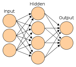 An neural network
 An NN dependency graph
 A single-layer feedforward neural network with 4 inputs, 6 hidden nodes and 2 outputs. Given position state and direction, it outputs wheel based control values.
 A two-layer feedforward neural network with 8 inputs, 2x8 hidden nodes and 2 outputs. Given position state, direction and other environment values, it outputs thruster based control values.
 Parallel pipeline structure of CMAC neural network. This learning algorithm can converge in one step.


.svg)


See also
- ADALINE
- Autoencoder
- Bio-inspired computing
- Blue Brain Project
- Catastrophic interference
- Cognitive architecture
- Connectionist expert system
- Connectomics
- Deep image prior
- Digital morphogenesis
- Efficiently updatable neural network
- Evolutionary algorithm
- Family of curves
- Genetic algorithm
- Hyperdimensional computing
- In situ adaptive tabulation
- Large width limits of neural networks
- List of machine learning concepts
- Memristor
- Mind uploading
- Neural gas
- Neural network software
- Optical neural network
- Parallel distributed processing
- Philosophy of artificial intelligence
- Predictive analytics
- Quantum neural network
- Support vector machine
- Spiking neural network
- Stochastic parrot
- Tensor product network
- Topological deep learning